Enriching Recommendation Models with Semantic IDs

TL;DR
This project explored using Semantic IDs (SIDs) with the HSTU model on MovieLens-1M and -20M. I show that simply replacing raw IDs with SIDs reduced model performance, but combining them showed hints of faster convergence. Analysis suggests SIDs may have limited values where collaborative behavioral signals dominate, but could remain promising for large-scale and content-driven domains.

Accompanying github code: github.com/shaox192/hstu-semantic-id

Hey there! Welcome to my first blog.

Here’s some context first if you are curious why someone with mostly psychology degrees suddenly become interested in this (feel free to skip if you just want the technical bits):

During my internship @NetEase YUANQI (which runs some of the leading social media platforms in China), I worked on improving both performance and efficiency of generative recommendation models. My project explored how to instill content understanding into generative recommenders and very happy to see clear gains in production. My experience there was so great that I decided to keep this as a hobby and continue to explore other ideas in my free time, which led to this toy project and this blog post.

I come from cognitive neuroscience, where we try to figure out how humans make sense of the world, and neuroAI, which aims to build artificial systems that understand and interact with the world in human-like ways. To me, recommender systems try to understand, model, and predict human behavior, which is, honestly, not so far from psychology’s goal.

What’s interesting to me is that, in practice, recommendation models often see posts or items as arbitrary IDs with additional engineered features that not alway aim to capture what the item is. However, you don’t need a Psychology degree to guess that the content of what someone interacts with (we call them “stimuli” in Psych) should matter a lot for predicting their behavior. With the emergence of semantic IDs in the field of recsys, I am curious to see how this interesting idea could change the traditional recommendatin paradigm, and more importantly, also ask why certain effects show up.

Disclaimer: Everything in this blog (and the accompanying repo) is based purely on open-source datasets and models. Nothing here is related to company IP.

What’s Wrong with Arbitrary IDs?

At a high level, recommendation systems take a user’s history — a sequence of posts, videos, products, or whatever depends on the platform — and try to predict what users will like next. The way we usually represent those items is by assigning each one an arbitrary ID and then retrieve the corresponding embeddings (or really learnable representation vectors) from a giant trainable embedding table we built during training. Simple enough. However, this setup has some well-known issues:

1. No sense of content: An embedding table doesn’t “know” that the post with ID “#1234jho1293da0kds” is a panda-having-bamboos-for-lunch video or ID “#hs2984fhdiuh339sd” is a review video for doctor who season 9. However, intuitively, making sense of what these posts are about should make the model’s job much easier.
2. Storage costs: The embedding table grows with the catalog or “item pool”. With millions (or billions) of items, the table gets massive and slow to index.
3. Meaningless Hash collisions: In reality, to save space, we often just host a fixed-size table and hash IDs into it, but then totally unrelated items can collide into the same slot, confusing the model.
4. The long-tail problem. Even if you can host a massive embedding table and avoid collisions, another problem is that most items, unfortunately, get very little training data because of the classic long-tail problem (You can take a peak at Figure 5 below that shows the long-tail problem for MovieLens): Usually, a small slice of popular items dominates the training data, because they’re genuinely fun or high quality. Their embeddings are therefore well trained, show up more often in recommendations, and (because they’re recommended more precisely) get even more positive interactions. –> A virtuous cycle for the lucky few.
   It is the opposite story for the vast majority of items in the long tail. They’re rarely seen, poorly trained, less likely to be recommended, and even when they do get recommended, the match is less precise, so they get fewer clicks, fewer likes, and stay stuck in the dark. –> A vicious cycle. However, many of those long-tail items could still be high quality and deeply interesting to someone. They just need a way to reach the right audience. In addition, encouraging the diversity is also critical to keep the platform vibrant, give users fresh content to explore, and motivates creators to keep contributing (the lifeline for UGC platforms).
5. Cold start for new items. On UGC platforms where hundreds and thousands of new posts are created every day, how do we assign meaningful embeddings to brand-new items without waiting for enough interaction data to accumulate?

And that’s where the idea of semantic IDs comes in.

Semantic IDs: What and Why

Semantic IDs (SIDs) turns out to align neatly with how modern LLMs use a fixed-size vocabulary to tokenize words and sentences. You may have run into this in generative recommendation systems like TIGER (Rajput et al., 2023), COBRA (Yang et al., 2025), LC-Rec (Zheng et al., 2024)…, and the popular end2end OneRec (Zhou et al., 2025). SIDs have quickly become the go-to trick in these models that treat a user’s interaction history as a sentence, and then performing NTP (next token prediction), or really NSP as in next SID-digit prediction in recsys settings.

The intuition behind SIDs is simple: each item gets relabeled with a tuple of numbers that capture different aspects of its content. For example, two pandas-eating-their-lunch videos might get SID [121, 23, 3] and [121, 23, 4]. The 121 could represent “panda”, while all videos with 23 at the second digit features some animals eating food. A doctor who season 9 review video, on the other hand, might get a quite different ID like [125, 0, 201]. Together, the digits form a compact code that hints at what the item is about.

So… how do we get these numbers?

1. Constructing SIDs

SID construction started with representation vector quantization (Hou et al., 2022), which clusters the entire item pool so that semantically similar items in the same cluster share an integer code. More sophisticated methods later built multi-digit tuples with Residual Quantized VAEs (RQ-VAEs), as in TIGER (Rajput et al., 2023). More recent work (e.g., OneRec (Zhou et al., 2025) and QARM (Luo et al., 2024)) uses k-means clustering. It’s much simpler than training VAEs, alleviating those training instabilities like latent space collapse and hourglass problems (Kuai et al., 2024), and still produces solid results.

Here’s the typical pipeline for generating SIDs:

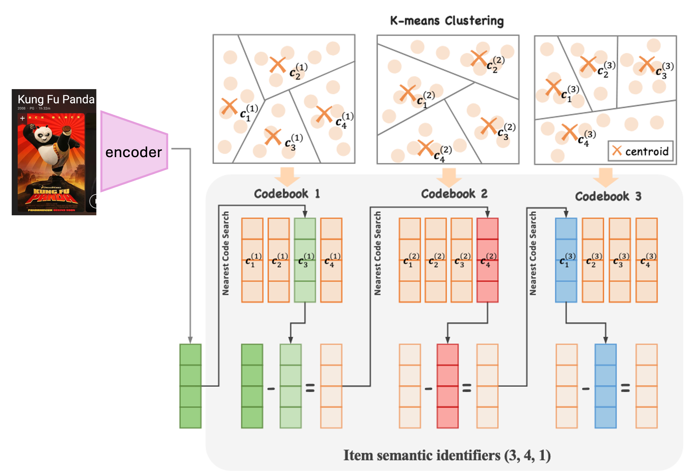Figure 1: Example pipeline for SID generation with RQ-kmeans, adapted from OneRec (Zhou et al., 2025).

1. Collect all items in your pool and generate their representations from your favorite encoder, e.g., LLMs for text posts, VLMs for multimodal posts, or fancy video models aligned with collaborative information (like OneRec).
2. Cluster them (say, into 256 groups) using k-means, VAE codebooks,or any methods you find appropriate, and assign each item its cluster ID. That fills in one digit of the SID tuple.
3. Compute residuals by subtracting each item’s embedding from its cluster center, then repeat step 2 to get the next digit.
4. Continue until you’ve reached the desired number of layers (or lengths of the SID).
5. Done! Every item now has a SID tuple.

The number of layers in the RQ procedure just means how many repetitions of step 2 and 3 you go through, and how many digits you get at the end. If you’ve ever worked with VAEs for image reconstruction in computer vision, the RQ procedure will feel familiar: each layer simply captures the leftover variance that wasn’t explained by the previous one. In a perfect theoretical world, we are able to recover the item by adding its corresponding cluster centroid representations.

Note: It seems that the more complex your dataset is, the more SID layers tend to help (Zheng et al., 2025, and see my analysis below near Figure 4), although usually I see numbers around 3 or 4.

Another note: You might have noticed that the numbers in a SID aren’t always meaningful by themselves. Whether 121 and 122 are semantically closer than 121 and 1000 depends entirely on the clustering method you used — and often, there’s no real ordering at all. Even if you pick a method that enforces some structure, once these IDs go into an embedding table, the model might still just see them as independent and different rows. In other words: the raw integers in SID don’t necessarily carry semantic distance on their own.

2. Are SIDs really hierarchical?

I sometimes see people describe SID codes as a hierarchy that goes from coarse to fine semantics. Although that sounds intuitive, it’s slightly misleading in that this suggests a conception similar to hierarchical clustering, where each deeper layer must 1. add finer details and 2. stay semantically tied to the previous layer.

However, with RQ clustering, each layer just captures the residual variance left over from the previous step, and that variance might have nothing to do with the earlier dimension. For example, layer 1 might separate videos by object type (pandas vs. dogs), while layer 2 splits them by language (Chinese vs. English). Which one is “coarser” or “finer”? Hard to say.

3. Why SIDs might be preferred

With SIDs, similar items share parts of their code: two panda videos might overlap on [121, 23, *]. Depending on how we eventually construct the SID embedding and feed into the model, these shared digits will give them similar embeddings, thus giving the model a better hint at user preferences.

More specifically, SIDs help address the earlier problems we discussed:

1. Meaningful IDs. Posts now have codes tied to their semantics.
2. Fixed embedding table. The size no longer scales with the item pool.
3. Long-tail boost. Less popular items can benefit from the training updates of popular ones that share their SID digits.
4. Cold start relief. New items can be clustered into existing SIDs right away, giving them a solid starting point.

Significance statement
You might think if SIDs are already used in all these generative recommender systems, why write another blog about them?

• First, no one seems to have tried this with HSTU, one of the most popular and influential generative recommender models.
• Second, I didn’t train HSTU to generate SIDs directly (as in NTP), but injected SIDs at the embedding level, while leaving the rest of the model unchanged. Here’s some pratical significance for going this route: most real-world recommenders today still have traditional architectures like two-towers doing the heavy lifting. These models are steady, efficient, and trusted at scale. Meanwhile, the industry’s (actually also academia’s) “generative everything” hype is already producing rich semantic embeddings for items. Finding ways to reuse those embeddings in classic systems could be a practical path to steady progress, and maybe also a way to gain insights into these new techniques.

Methods

1. Model

I chose to focus on HSTU (Zhai et al., 2024), a transformer-based sequential recommender for retrieval. At a high level, it works just like language models: it takes in a user’s history sequence and predicts the next item. There are lots of clever details in the paper that make HSTU both powerful and efficient, and I recommend reading it if you’re curious. For our purposes, the key setup that need to be clarified before diving into the details later is as follows:

• The model maintains an embedding table for all items (based on their arbitrary IDs).
• Given a user history, the model produces a final embedding.
• At prediction time, that embedding is compared against all item embeddings in the table (for example, using a simple inner product), and the most similar item is retrieved.

2. Data

Experiments were run on the classic MovieLens-1M and MovieLens-20M datasets (here). These are great benchmarks, but out of the box they’re pretty much barebones: just a title, release year, and a couple of genre tags for each movie, so do not include rich semantic information.

To make them more appropriate for semantic IDs, I built an extended version of MovieLens-1M and MovieLens-2M with additional metadata pulled across various sources that includes plot synopses, long keyword lists, language/nationality tags, some featured reviews and other details. These allowed me to put together a rich description and fed into a text encoder (I used qwen3-0.6B) to obtain the embeddings.

Extended MovieLens: full details and download links are also in the accompanying git repo.

3. Building and embedding SIDs

I used RQ-k-means to build SIDs, so at each layer, I clustered the items with k-means and produced a tuple of integers for every item using residual quantization steps outlined above.

As discussed in the previous section, we ended up with a tuple of integers as semantic IDs for each post. Since we are not generating each digit of SID as with NTP, but instead finding the next item by embedding similarity, then the key question is:

How do we turn a SID tuple into an embedding?

Most of options that I tried require setting up a fixed size embedding table, performing some transformations on the SID tuples to obtain one, or multiple rows from the embedding table, and then pooling these rows to obtain the final embedding.

Now let’s say that we have a fixed size SID embedding table with N rows, and we have SIDs with L layers and C codes per layer (thus having SIDs like: \([c_1, c_2, …, c_L]\)). Then some possibilies are:

3.1. N-gram

If we think of a SID tuple as a “sentence”, we can borrow this n-gram ideas from NLP. One example is that if we use the entire tuple as an L-gram. We then map it into a single integer using some common positional encoding scheme:

This works, but if the SID combinations are fine-grained, many tuples will be unique, and we’re back to the “arbitrary ID” problem, so we are not really leveraging the advantage of the SIDs.

A better approach would be using multiple smaller n-grams (e.g., bigrams) and then pool the corresponding embeddings. The question is: are bigrams enough? Should we also throw in unigrams, trigrams…, all the way up to L-grams? You can see how this quickly gets messy. The nice thing is that tokenization is already a very widely studied problem in earlier years of NLP. We can borrow those ideas here and, for example, use smarter methods like SentencePiece (Singh et al., 2024) to decide what the best “units” of n-grams should be.

3.2. PrefixN

One appealing solution is PrefixN (Zheng et al., 2025). The idea is to extract multiples rows from the embedding table, each based on the prefixes of different lengths of SID digits. For example, for the SID: \([c_1, c_2, …, c_L]\), we need to extract the following rows from the embedding table:

• Row \(c_1\)
• Row \(C^1 \cdot c_1 + c_2\)
• Row \(C^2 \cdot c_1 + C^1 \cdot c_2 + c_3\)
• …
• Row \(C^{L-1} \cdot c_1 + C^{L-2} \cdot c_2 + \dots + c_L\)

and then pool these embeddings together with summation.

Note Although I noted above that it seems the more layers and more codes we use for SIDs, the better for the performance, this really depends on dataset. For both MovieLens-1M (~3.8K items) and -20M (~28K items), the amount of useful information for prefixes diminishes quickly. See my analysis below.

Another note Prefix N deviates a little, conceptually, from the how SIDs are built with RQ-cluster methods. It really hints at the hierarchical dependency, and as I mentioned above, in RQ-cluster settings, layers capture residual variance, not a clean semantic hierarchy as in a real language setting.

3.3. RQsum

Then there is the RQsum approach which, I suppose, stays closest to the spirit of RQ methods in their original use cases like image reconstruction: that is, each SID digit corresponds to a quantized cluster centroid and if we sum those centroids, we can approximately reconstruct the original item embedding.

Concretely, RQsum builds a small embedding table with size \(L \times C\), meaning that each digit in the SID tuple has its own embedding, and we simply sum these embeddings together to represent (or, reconstruct) the semantics of the item.

This is intuitive, simple, and aligns with how RQ-based representations were originally designed.

4. SID Embeddings + Individual IDs

I will save the full story for the results section, but here’s one important setup that I tried. Instead of replacing the original arbitrary item IDs with semantic IDs, we can keep both the original ID embeddings and the SID embeddings, and then fuse them together.

Why? Aren’t we throwing away all those efficiency benefits from using SIDs? Well, on both MovieLens-1M and 2M, using SIDs alone actually hurt performance by quite a bit (see my results section below). In other words, they were not sufficient to support the task by themselves. My hunch, as I will discuss later, is that MovieLens is a dataset driven by collaborative behavioral signal rather than the detailed semantics of movies. SIDs may have just blurred the behavioral signals that the model needed to capture sharply.

So the natural next question was: what if we add SIDs as extra information instead of replacements? Even if they’re not precise enough alone, they might give the model a jump-start during training by sharing embeddings and act as an informative prior for the raw IDs to bring additional benefits.

To fuse them together, I tried a few approaches:

• Simple sum pooling: just add the ID embedding and the SID embedding.
• Weighted pooling: learn a parameter \( \alpha \) so the final embedding is \( \alpha E_\text{SID} + (1 - \alpha) E_\text{ID} \).
• More complex methods available to try in my code repo: like FC layers, MLPs, or scalar/vector gating. (Spoiler: these mostly hurt performance by introducing too many extra parameters.)

With this setup in place, we can now move on to take a look at how SID-augmented HSTU actually performs.

Results – Do SIDs Help?

Sadly, although interestingly, replacing arbitrary IDs entirely with SIDs made things worse (Figure 2 prefixN condition). With both ML-1M and ML-20M, performance dropped sharply. I am showing MRR here, but the overall trends and differences are consistent for other metrics like hit rate and NDCG.

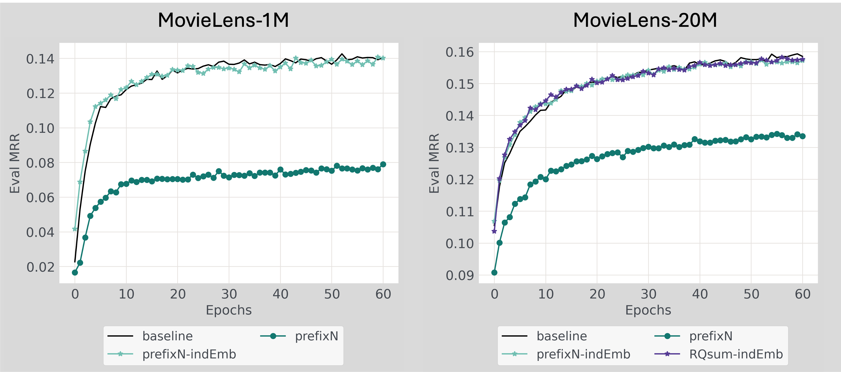Figure 2: Model performance (MRR) on MovieLens-1M (left) and MovieLens-20M (right). baseline: Vanilla HSTU model with arbitrary IDs only. prefixN: HSTU with arbitrary IDs entirely replaced with PrefixN-based SID embeddings. prefixN-indEmb: HSTU model with PrefixN-based SID embeddings combined with original ID embeddings using sum pooling (ML-1M) or learnable alpha weight (ML-20M). RQsum-indEmb: Similar to prefixN-indEmb, but used RQsum method to construct SID embeddings.

As I briefly mentioned in the previous methods section, this is what led me to consider using SIDs alongside the original IDs, as an additional prior. I tried both PrefixN and RQsum embedding construction methods in this hybrid setup (prefixN-indEmb and RQsum-indEmb conditions in Figure 2). Interestingly, it seems that:

• Early in training, SID-augmented models showed a small but visible advantage, hinting that embedding sharing through SIDs might help convergence.
• But the effect quickly faded, and by later epochs the models with SIDs weren’t noticeably better than the baseline (slightly worse, if we look closely at the exact numbers).

Why SIDs did not work as expected? Below I show a few analyses that might shed some light on this.

Analysis - Diagnosing the data and model

1. Do SIDs Roughly Predict User Preferences?

The first thing I needed to check was: do my SIDs make sense? In other words, for a given user, do the movies in their history share similar SID prefixes or digits, or are they simply scattered randomly (which would suggest that movie content, or at least that captured by my SIDs here, do not reflect users’ preference in this context at all)?

To check this, I measured how often prefixes (and single digits) repeat within each user’s history. For each user, I counted the proportion \(p_{uniq}\) of unique prefixes (or digits), and then took \(1 - p_{uniq}\) to get a measure of commonness (higher = more overlap).

I ran this analysis for both MovieLens-1M (Figure 3) and ML-20Ms (Figure 4):

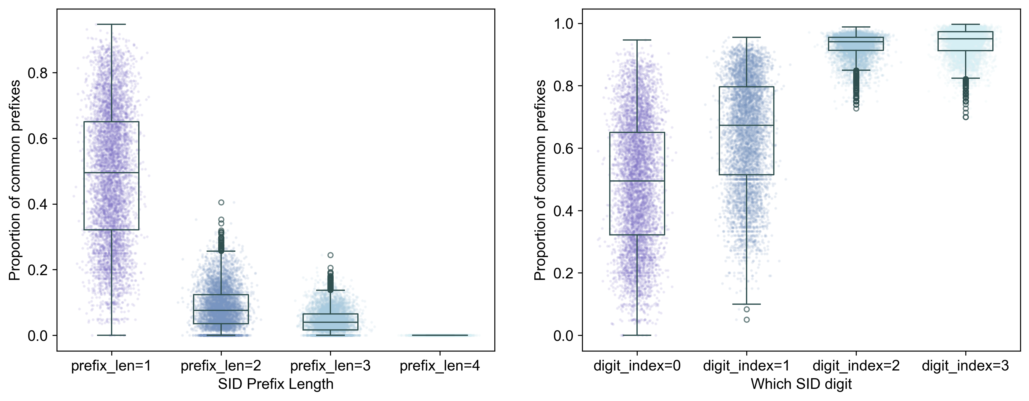Figure 3. Distribution of propotion of common SID prefixes (left) and digits (right) for MovieLens-1M. Each dot = one user. Higher values = more movies share the same SID prefixes or digits, thus indicating that SID is more predictive of that user’s history.

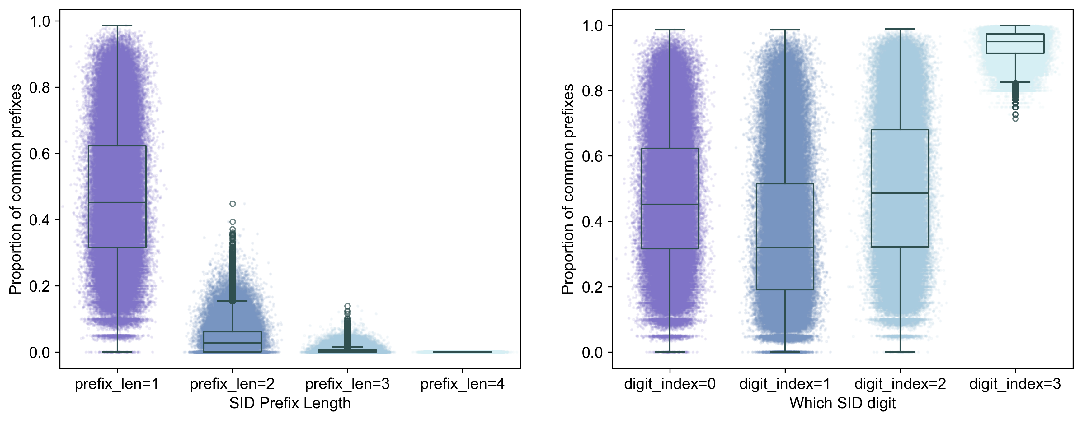Figure 4. Distribution of proportion of common SID prefixes (left) and digits (right) for MovieLens-20M.

We see that:

1. SIDs roughly predicts user history: Shorter prefixes and single sigits show that at least for half of the users, half of the moviews they have watched share similar content. Longer prefixes are more fine-grained, so they naturally become less predictive of a user’s history. However, there is also a large portion of users for whom SIDs do not reflect well their histories.

Note In my setup, I added an extra layer that makes each full-length SID unique (like TIGER does). That means with prefix_len = 4, SIDs for all movies become entirely unique, and thus we see floor values in, for example, Figure 3, left, prefix_len=4 group. In the single-digit plots, on the other hand, the last digit hit ceiling values because the final layer just assigns 0, 1, 2, … to distinguish otherwise identical SIDs (TIGER style).

1. SID collapses for smaller datasets even with k-means In ML-1M, layer 3 (digit index 2) also hit ceiling values. Does that mean it’s “special” and magically fully overlaps with user history? Not really — it’s a collapse with k-means. That layer only formed two major clusters, making it appears perfectly predictive. This collapse didn’t happen in ML-20M, which suggests that increasing the depth (more layers) of SIDs is only meaningful on richer, larger datasets.

Regardless, SIDs should not be totally useless or misleading. More specifically, two SID digits seem informative for MovieLens-1M, while three digits are useful for MovieLens-20M, roughly speaking.

2. Do SIDs Help with the Long-Tail Problem?

One of the big promises of semantic IDs is that they should help long-tail items — the less popular movies that don’t get enough data to train strong embeddings. By sharing SID embeddings with semantically similar but popular items, tail items could, in theory, ride along and get better recommendations.

Although I didn’t see much overall improvement in overall model performance as shown in the previous results section, SID-augmented models did show a tiny, but definitely visible, initial advantage, suggesting that embedding sharing may indeed be beneficial. This made me wonder: maybe the effect is different for popular and long-tail items, and the differences cancel out at the aggregate level?

The hypothesis would then be: SID augmented models should perform better than baselines for long-tail items as a results of embedding sharing, but may lag behind with popular items, potentially because the imperfect SID signal only misleads the model while the rich behavioral data alone can send a clear signal already.

2.1 The long tail is real

First, here’s the impression distribution:

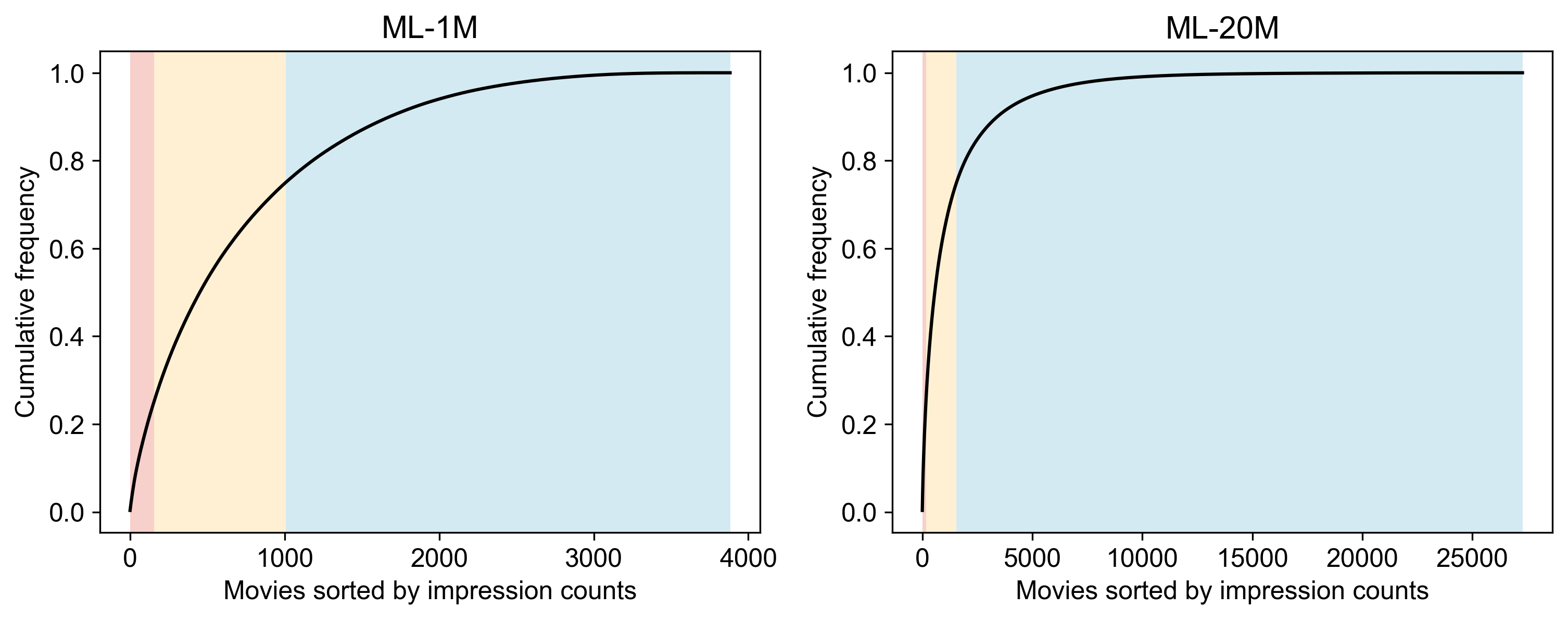Figure 5. Impression distribution in ML-1M (left) and ML-20M (right). Movies are sorted by impression count; the top 25% are the popular items colored in red (hot items), middle 50% are colored by yellow (mild items), and bottom 25% are the long-tail items colored in blue (cold items)

We see that:

• In ML-1M, just 154 out of 3.8K movies contribute 25% of all impressions.
• In ML-20M, 164 out of 28K movies contribute 25% of all impressions (an even steeper long tail).

So the long-tail problem is definitely present, and stronger in ML-20M.

2.2 Performance by bins

Now following Zheng et al. (2025), I split movies into three bins:

• Hot (0–25%): the most popular items
• Mild (25–75%): the middle majority
• Cold (75–100%): the long-tail items

Then I compared the performance of baseline HSTU with SID-augmented HSTU (prefixN-indEmb models), both trained on the same entire training set, in each bin. On MovieLens-1M, we see this:

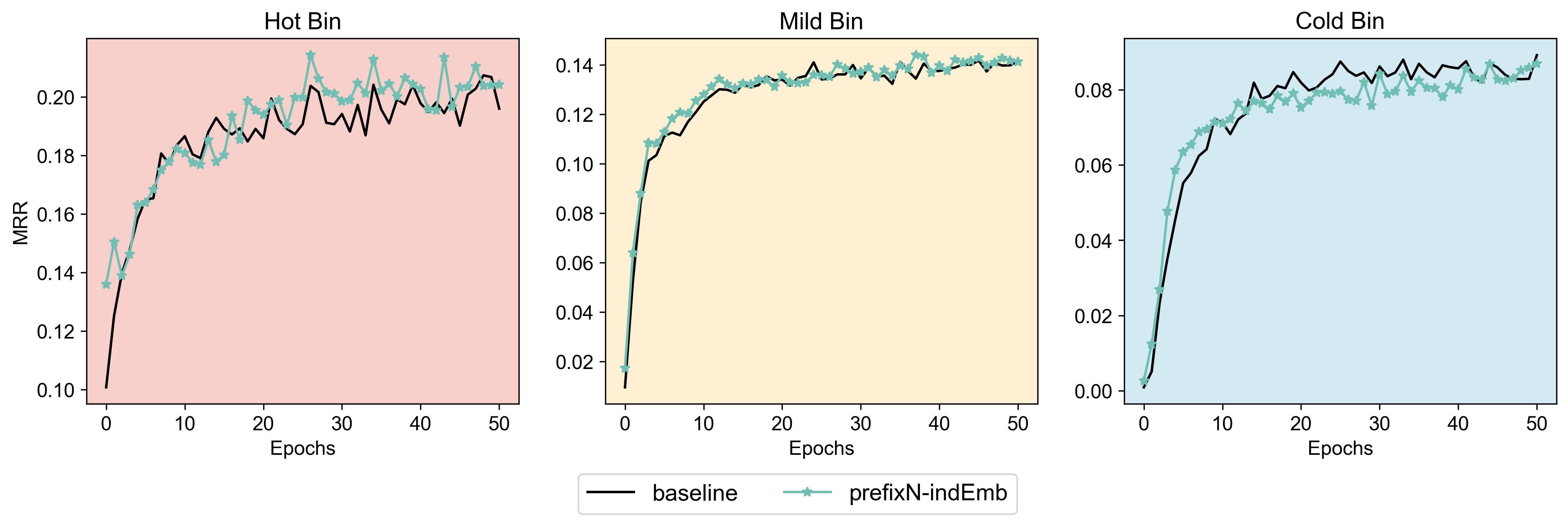
Figure 6. ML-1M: MRR across popularity bins for baseline vs. SID-augmented model.

• Cold bin: SID shows an early boost but performance drops later in training.
• Hot bin: interestingly, SID helps later in training, but there is no initial advantage.
• Mild bin: basically no effect.

This seems to suggest that SID do bring additional benefits compared to using arbitrary IDs, in that there is an advantage of embedding sharing in the beginning for the long-tail items, although they soon turn into a burden. On the other hand, SID seemed to help with the popular items later on. However, before jumping into interpretations, does this result replicate with ML-20M dataset? Not really.

With ML-20M (Figure 7), we see this:

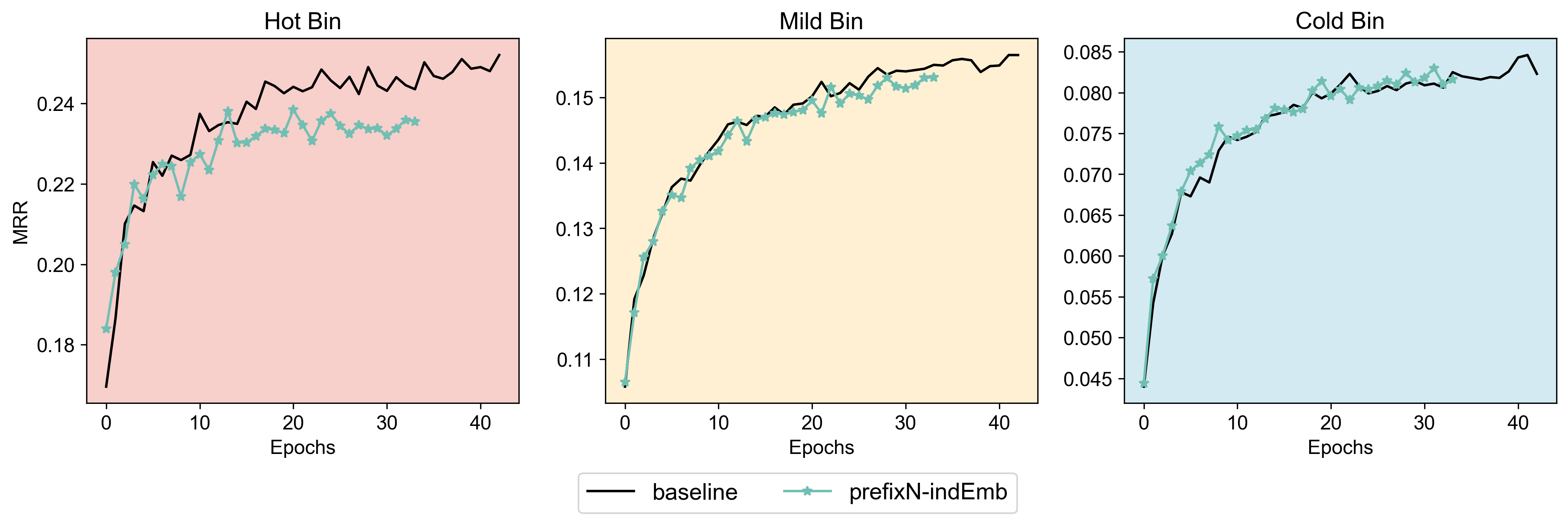
Figure 7. ML-20M: MRR across popularity bins for baseline vs. SID-augmented models.

• Hot bin: SID started to hurts performance despite the initial jumps.
• Mild + Cold bins: no clear effect either way.

So it seems that the story is not entirely straightforward: while the “SID should fix the long-tail problem” idea is appealing, these analyses suggest the effect might be dataset-dependent. At least on MovieLens, SIDs don’t cleanly solve the problem.

Final thoughts

Taking everything together, replacing raw IDs with SIDs seems to be a bad idea, and using them as an extra prior only gave small early boosts. But I don’t think this means SIDs are useless, rather it says more about the datasets and models in my setup than the concept itself:

1. What drives preferences matters.
   The key question is: are user choices driven more by content or by collaborative behavior (that is, “people who liked this also liked that”)?
   For movies, the answer seems to lean heavily toward the latter. Yes, I prefer sci-fi and try my best to avoid horror movies, but what I actually watch next usually depends on social proof (what is in the “Top rated” list under the sci-fi genre). In this setting, fine-grained content features may add much more benefit and can even distract the model from the rich behavioral signal.

2. Data Scale matters.
   On ML-1M, the training data scale may not be rich enough for the item pool, so SID overlap helps a little at the start. On ML-20M, with 7× more items but 20× more behavioral data, collaborative signals could very well dominate. Coarse SID “sharing” this time just adds noise to an already strong signal.

3. Model strength matters.
   HSTU is already a very strong sequential recommender. Since SIDs are lossy approximations of item semantics (and also highly depend on the quality of the embeddings), much of the variance they capture can be inferred by the model already from behavior alone.

4. Implementation and engineering matters
   There are, more than likely, better ways to generate SID embeddings and fuse them with raw IDs. My encoder wasn’t huge (limited by my poor but very hard-working 4090), and my fusion strategies were simple. Smarter encoders, prompts, or fusion methods might unlock more benefits.

Well then where could SIDs be useful? It seems to me that the more promising scenarios are those with huge, fast-changing item pools and content-driven user behaviors. Consider UGC platforms like TikTok or Instagram Reels, where what matters is the content of the post, and new items appear every second. Or maybe research paper recommendation, where the catalog grows everyday and choosing what to read depends almost entirely on topic relevance.

Thanks for reading! I hope this post was helpful or at least sparked some ideas.

If you have thoughts, questions, or want to chat about recommenders and semantic IDs (or my day job cognitive neuroscience), feel free to reach out! I would love to hear from you.